Datadog NetFlow Monitoring with FluentD

I recently worked on an interesting assignment where NetFlow monitoring was needed for network traffic analysis. Now, the Datadog platform has a rich feature set for analyzing and visualizing just about any type of data, and NetFlow is no different.

The only unusual aspect of the assignment was with collection; We’ll need to use the open source FluentD to collect NetFlows, so in this post I’ll share how FluentD can be used to collect flows for analysis on the Datadog platform.

Brief Overview

I’ve not had a chance to work with FluentD previously, though I’ve heard good things about it. What’s useful about the FluentD agent is that it is modular and extensible with plugins. Particularly, it has both a Netflow Collector source plugin and the Datadog output plugin, which we need. Fun fact, the NetFlow plugin is a certified FluentD plugin, while the Datadog plugin is directly maintained by Datadog developers!

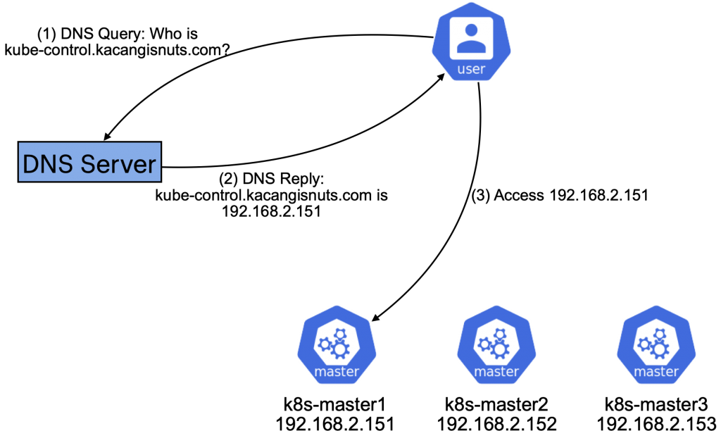
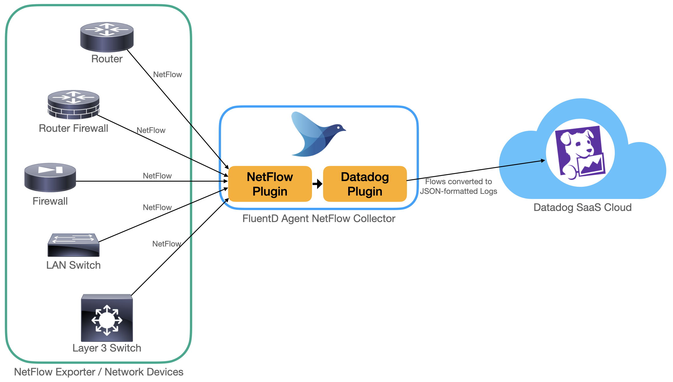
With both of these plugins available, it becomes a matter of configuring FluentD as a NetFlow collector, which will then convert flows to JSON-formatted logs to be submitted to Datadog. It’s really as simple as the diagram below.

The big picture: How FluentD collects and send NetFlows to Datadog

Getting Started

We use a vanilla Ubuntu 18.04 LTS VM, and install the pre-compiled FluentD agent like so:

$ curl -L https://toolbelt.treasuredata.com/sh/install-ubuntu-bionic-td-agent4.sh | sh

This installs the latest FluentD agent, and automatically configures systemctl to start it as a service. In case you’re using some other Linux distro, pop over to the FluentD Installation page and follow the distro-specific instructions. I’ve tested a similar set up with RHEL 7, and that works flawlessly too.

Once done, run a quick systemctl check to ensure that the agent is up and running:

$ sudo systemctl status td-agent
● td-agent.service - td-agent: Fluentd based data collector for Treasure Data
   Loaded: loaded (/lib/systemd/system/td-agent.service; enabled; vendor preset: enabled)
   Active: active (running) since Sun 2021-04-11 10:20:00 UTC; 15s ago
     Docs: https://docs.treasuredata.com/articles/td-agent
  Process: 17416 ExecStart=/opt/td-agent/bin/fluentd --log $TD_AGENT_LOG_FILE --daemon /var/run/td-agent/td-agent.pid $TD_AGENT_OPTIONS (code=exited, status=0/SUCCESS)
...

That all looks hunky dory, but what on earth is all that td-agent business, you ask? It turns out that the company Treasure Data maintains most (all?) stable distribution packages of FluentD. Hence, the FluentD agent is called td-agent in these distributions. You can read more about it in the official FluentD FAQ, but suffice to say that td-agent is equivalent to FluentD for our purposes. Keep in mind though, this does mean that command names, configuration files, etc will carry the td-agent name instead.

Installing the NetFlow Collector Source Plugin

Here, we install the Netflow plugin for FluentD, which turns the FluentD agent in to a NetFlow Collector. Run the following command to install the plugin:

$ sudo /usr/sbin/td-agent-gem install fluent-plugin-netflow

Insert the following lines into /etc/td-agent.conf. I use UDP port 5140 to receive flows in my lab, though you can change this to other ports if you like. Remember to point the NetFlow Exporter to the right UDP port later.

<source>
  @type netflow
  tag datadog.netflow.event
  bind 0.0.0.0
  port 5140
  versions [5, 9]
</source>

If you notice, we’re tagging all flows with datadog.netflow.event. This tag will be used by FluentD to match and route the flows to the appropriate plugin for handling. The ‘next steps’, so to speak.

Installing the Datadog Output Plugin

Next, we install the Datadog plugin that will transport the flows as JSON logs to the Datadog cloud for processing and analytics.

$ sudo /usr/sbin/td-agent-gem install fluent-plugin-datadog

Add the following lines into /etc/td-agent.conf, BELOW the NetFlow plugin configuration from the last section, and insert your Datadog API key at the api_key parameter.

<match datadog.netflow.**>
  @type datadog
  api_key <API KEY>

  dd_source 'netflow'
  dd_tags ''

  <buffer>
    @type memory
    flush_thread_count 4
    flush_interval 3s
    chunk_limit_size 5m
    chunk_limit_records 500
  </buffer>
</match>

There are some interesting points about this configuration. Notice first that the match directive looks for datadog.netflow.**. The ** bit is a greedy wildcard, and causes the plugin to process any flows with a tag starting with datadog.netflow. That includes flows collected by the NefFlow plugin, which we earlier configured to apply a datadog.netflow.event tag.

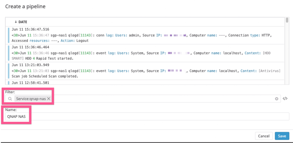
Secondly, notice that dd_source 'netflow' is set, ensuring that flows have the tag source:netflow. It is Datadog’s best practice to use to the source tag as a condition to route logs (flow logs in this case) to the appropriate log pipeline after ingestion. The pipeline then processes, parses and transforms log attributes. Where possible, the pipeline also performs enrichment, for example adding country/city of origin based on a source IP address. This is actually a whole big topic on its own but suffice to say, it is important to configure the source tag appropriately.

Finally, there’s also the ddtag parameter which isn’t used in the example here. This allows the application of custom tags, which could be useful in a larger environments. For example, a large enterprise may have different NetFlow collectors for different zones (DMZ, Internet gateways, branches, data centers, just to name a few), different sites, different clouds etc. Being able to drill into a specific collection context or view using tags is handy to gain extra clarity during analysis.

Now that we’re done with configuring the FluentD agent, make sure to restart the service so the changes take effect.

$ sudo systemctl restart td-agent

Configuring pfSense as a NetFlow Exporter

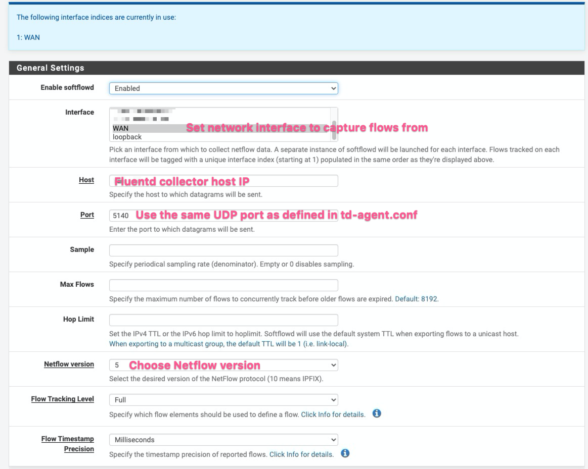
Configuring a network device as a NetFlow Exporter differs depending on the device. In my case, I use a pfSense firewall as my NetFlow exporter. There are more detailed instructions on installing and enabling NetFlow for pfSense using the softflowd plugin, so we won’t go into the details here.

As a sample configuration however, here is how softflowd is set up on my pfSense firewall to export flows. In short, these settings configure the firewall to collect flows traversing the WAN interface, and then to send them as Netflow v5 flows to port 5140 of the FluentD NetFlow Collector.

pfSense softflowd config in a nutshell

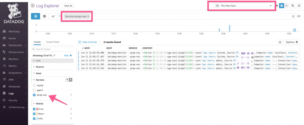
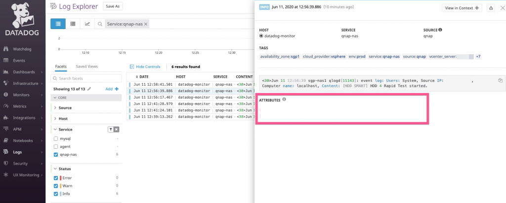
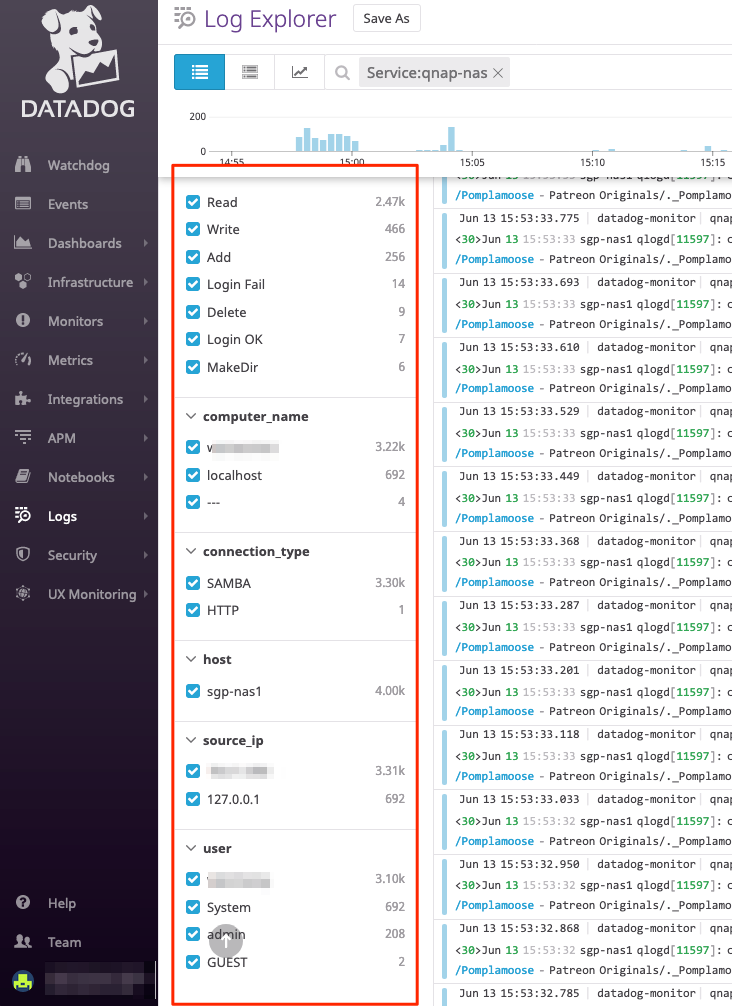
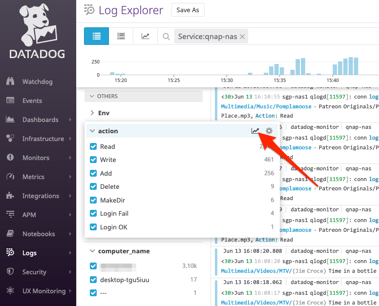
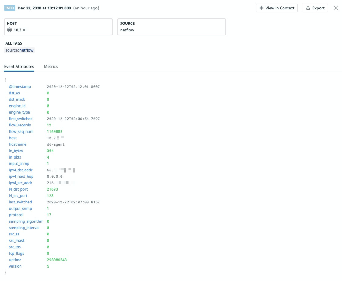
Assuming everything works as advertised, logging into the Datadog Log Explorer screen shows all the NetFlow flow logs that are collected. Popping open any of the flow logs shows the various attributes that were parsed from the flow logs. Unmistakably, the really important ones like Source IP, Source Port, Destination IP, Destination Port, Protocol type, as well as Bytes and Packets transferred are all available.

NetFlow ingested as JSON

Quick Peek at the NetFlow Dashboard

In the interest of keeping this post on topic around FluentD NetFlow collection, we’ll cover Datadog logs processing some other time. However, as a peek into the possibilities once we’ve got flows ingested, processed and analyzed, here’s a really groovy NetFlow monitoring dashboard that I created.
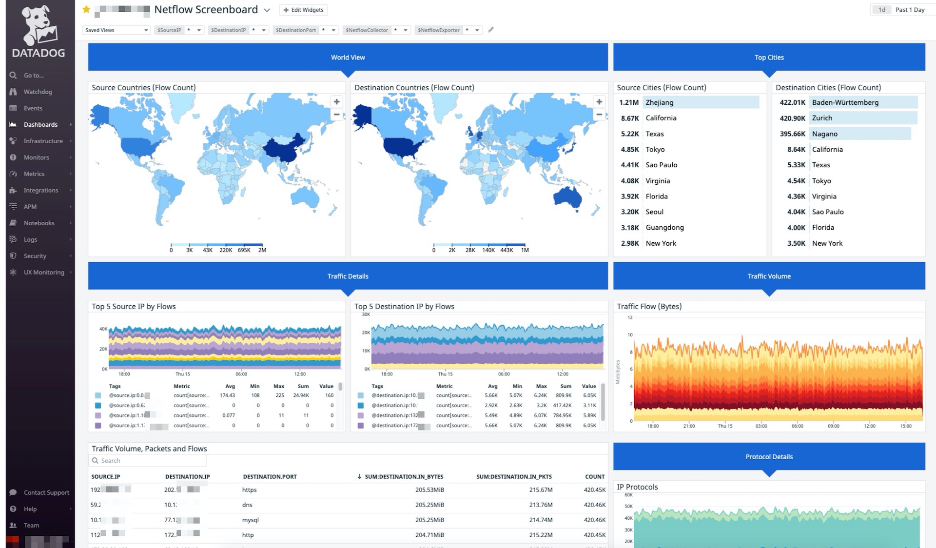
One global NetFlow Dashboard to rule the world

Neat, isn’t it?

Kubernetes Control Plane Resiliency with HAProxy and Keepalived

I had a bit of fun setting up an on-premise Kubernetes cluster some time back, and thought I’d share an interesting part of the implementation.

Briefly, today’s post describes how to set up network load balancing to provide resiliency for the Kubernetes control plane using HAProxy. To ensure that this does not create a single point of failure, we’ll deploy redundant instances of HAProxy with fail-over protection by Keepalived

Brief Overview – Wait, the what and the what, now?

A production Kubernetes cluster has three or more concurrently active control plane nodes for resiliency. However, k8s does not have a built-in means of abstracting control plane node failures, nor balancing API access. An external network load balancer layer is needed to redirect connections to the nodes intelligently during a service failure. At the same time, such a layer is also useful to distribute API requests from users or from worker nodes to prevent overloading a single control plane node.

The diagram below from the Kubernetes website shows exactly where the load balancer should fit in (emphasis in red is mine).

By the way, I definitely did not figure all this out on my own, but started by referencing the rather excellent guide at How To Set Up Highly Available HAProxy Servers with Keepalived and Floating IPs on Ubuntu 14.04, then adapting the instructions for load balancing k8s API servers on-premise instead.

Initial DNS and Endpoint Set Up

To make this work, you need a domain name and the ability to add DNS entries. It’s not expensive, a non-premium .org or .net domain costs about USD13 per year (less during promotions). It is useful to have a domain for general lab use, and for experiments like what we are doing here. Of course, if you’ve got an in-house DNS server with a locally-relevant domain, that’ll work as well.

Whichever DNS service you go with, choose an fully-qualified domain name (FQDN) as a reference to your k8s control plane nodes. For example, I own the domain kacangisnuts.com, and would like my k8s control plane API endpoint to be reachable via the FQDN kube-control.kacangisnuts.com.

The steps to map the FQDN to an IP will differ by registrar. To start off, map the FQDN to the first k8s control plan node’s IP. We will update this later, but it is important to start with this to initialize the control plane. The mapping I use in my lab looks like the following:

  • DNS Record Type: A
  • DNS Name / Hostname: kube-control
  • IP Address: 192.168.2.151

With this DNS entry in place, all connectivity to kube-control.kacangisnuts.com goes to the first control plane node.

Initial DNS setup

At this point, set up the first and subsequent control plane nodes using the instructions at Creating Highly Available clusters with kubeadm. This post won’t go into the details of setting up the k8s cluster, as it’s all in the guide. A key point to note is that the FQDN to use as the k8s control plane endpoint must be explicitly specified during init. During my lab setup, that looks like:

kubeadm init --control-plane-endpoint=kube-control.kacangisnuts.com

Updating DNS and Configuring HAProxy Load Balancing

To get resiliency on the Control Plane, we will insert a pair of HAProxy load balancers to direct traffic across the control plane nodes. At the same time, we want to make use of health-checks to identify failed nodes, and avoid sending traffic to them.

Also, to avoid the load balancer layer itself becoming a single point of failure, we’ll implement load balancer redundancy by making use of Keepalived to failover from the Master HAProxy to the Backup HAProxy if a failure occurs.

At the end of the setup, we should have the following in place:

End state with load balancing and redundancy

To start, first modify the DNS entry for kube-control.kacangisnuts.com to point at the Virtual IP that will be used by HAProxy pair.

  • DNS Record Type: A
  • DNS Name / Hostname: kube-control
  • IP Address: 192.168.2.140

Set up two Linux instances to be redundant load balancers; I used Ubuntu 18.04 LTS, though any distro should work as long as you can install HAProxy and Keepalived. We’ll call these two haproxy-lb1 and haproxy-lb2, and install HAProxy and Keepalived on both like so:

sudo apt install haproxy keepalived

Without changing the default configs, append the following frontend and backend config blocks into /etc/haproxy/haprox.cfg for both haproxy-lb1 and haproxy-lb2:

frontend k8s-managers.kacangisnuts.com
        bind *:6443
        default_backend k8s-managers

backend k8s-managers
        balance roundrobin
        mode tcp
        default-server check maxconn 20
        server k8s-master1 192.168.2.151:6443
        server k8s-master2 192.168.2.152:6443
        server k8s-master3 192.168.2.153:6443

This configuration load balances incoming TCP connections on port 6443 to the k8s control plane nodes in the backend, as long as they are operational. Don’t forget to restart the haproxy service on both load balancers to apply the config.

$ sudo systemctl restart haproxy

Configuring Keepalived for Load Balancer Resiliency

Keepalived will use the Virtual Router Redundancy Protocol (VRRP) to ensure that one of the HAProxy instances will respond to any requests made to the Virtual IP 192.168.2.140 (which, if you remember, we mapped kube-control.kacangisnuts.com to previously).

The following are configurations that need to be set at /etc/keepalived/keepalived.conf for the respective load balancer instances. There are slight differences between the configs of the nodes, so be sure to apply them to the correct nodes.

# For haproxy-lb1 VRRP Master

vrrp_script chk_haproxy {
    script "pgrep haproxy"
    interval 2
    rise 3
    fall 2
}

vrrp_instance vrrp33 {
    interface ens160
    state MASTER
    priority 120

    virtual_router_id 33
    unicast_src_ip 192.168.2.141
    unicast_peer {
        192.168.2.142
    }

    authentication {
        auth_type PASS
        auth_pass <PASSWORD>
    }

    track_script {
        chk_haproxy
    }

    virtual_ipaddress {
        192.168.2.140/24 dev ens160 label ens160:1
    }
}
# For haproxy-lb2 VRRP Backup

vrrp_script chk_haproxy {
    script "pgrep haproxy"
    interval 2
    rise 3
    fall 2
}

vrrp_instance vrrp33 {
    interface ens160
    state BACKUP
    priority 100

    virtual_router_id 33
    unicast_src_ip 192.168.2.142
    unicast_peer {
        192.168.2.141
    }

    authentication {
        auth_type PASS
        auth_pass <PASSWORD>
    }

    track_script {
        chk_haproxy
    }

    virtual_ipaddress {
        192.168.2.140/24 dev ens160 label ens160:1
    }}

Very briefly, the vrrp_script chk_haproxy config block defines that Keepalived should first check and ensure that the haproxy process is running, before the load balancer node can be considered as a candidate to take up the virtual IP. There’s no point for a load balancer node to take up the Virtual IP, and not have a HAProxy operating to process connections. This check is also a fail-over criteria; if a load balancer node’s haproxy process fails, then it should give up the Virtual IP so that the backup load balancer can take over.

In the vrrp_instance vrrp33 block, we define the fail-over relationship between the two load balancer nodes, with haproxy-lb1 being the default active instance (with higher priority), and haproxy-lb2 taking over only if the first instance fails (lower priority). Note that the virtual IP is also defined here; This is the IP address identity that the active load balancer will assume to service incoming frontend connections.

Finally, restart the keepalived service on both nodes once the configs have been saved:

$ sudo systemctl restart keepalived

Peace of Mind

Well, that was somewhat involved, but we’re done. With this in place, barring a catastrophic outage, users using kubectl and k8s worker nodes configured to reach the control plane endpoint via FQDN / Virtual IP will not be affected by any single component failure at the Control Plane layer.

Part 2: Setting up Log Analytics on Datadog for QNAP NAS

In Part 2, we walk-through how to set up log parsing in Datadog for the QNAP NAS logs that the Datadog agent has been shipping out. This is an important step to allow filtering logs for troubleshooting, as well as creating facets for slicing, dicing and analyzing log data.

If you haven’t read Part 1: Setting up Log Analytics on Datadog for QNAP NAS yet, and arrived at this post without any clue as to how you got here, I highly recommend starting there.

To make your experience of this post better, here are some tips:

  • There are a number of screenshots in this post which may seem a bit small on their own. Click on them to pop-up a lightbox with an enlarged image. No, you don’t need a magnifying glass.
  • For easy understanding, we’ll split this out into the “Before”, “Setting Up”, and “After” sections.

Before Parsing Custom Logs

On the Datadog platform, navigate to Logs -> Search to get to the Log Explorer. Select only the qnap-nas Service facet. If you remember from Part 1, we had this Service configured on the agent configuration file. It might be a good idea to choose a longer time frame to view logs; In this case, we looking at logs from the “The Past Hour”. To generate some log activity, I logged into my NAS to start an antivirus scan as well as run a rapid test on one of the hard disks.

Yay logs.

Clicking into any of the log lines, it’s soon clear that while the logs exist, the data is not actually parsed for easy slicing and dicing, which will be immensely useful if we want to perform log analysis and filtering. It would be nice to extract inline data into easy to use attributes.

No attributes, no fun.

Setting Up Custom Log Parsing

Navigate to Logs -> Configuration. Obseve that there are already a number of existing log parsing pipelines which come out of the box (Wait, do we have boxes for a SaaS?). These are automatically turned on when an associated monitoring integration is enabled. Did I mention that Datadog has 400+ vendors-supported integrations already available, and chances are that whatever you want to integrate for monitoring/tracing/log analytics is already here? Consider it said 🙂 And now, lets add on a custom log pipeline, just cuz we can. Click on “Add a new pipeline”.

To add a new log pipeline, click on “Add a new pipeline”. Whew, how hard was that?

First, we need to filter out log lines that we want to send through our QNAP log pipeline for parsing. We’ll simply use service:qnap-nas as our filter criteria. If you recall, we configured the agent in Part 1 to tag this attribute to all logs that come in from the QNAP NAS. Give this pipeline an easily distinguishable name; “QNAP NAS”, for example.

I call the pipeline “QNAP NAS”, just because.

Once the pipeline exists to snag the right logs, we need to apply some actions to the logs in order to parse it. In this case, the actions are called “Processors”. Click on “Add Processor”.

Add a “New Processor”, professor.

A pop-up appears to help configure the “New Processor”. For Step 1, let’s leave it as the default “Grok Parser”, because we are going to use Grok to extract attributes of interest. In Step 2, return to the “Log Explorer” screen to copy out a few log samples which will be used to test our parsing rules. From observation, there appear to two types of QNAP NAS logs; An event log type and a connection log type. Notice that all of the log samples have a red “No Match” indicator next to them, meaning we can’t extract any useful attributes yet.

Copy and paste in some sample logs from the QNAP NAS so we can test the Grok parsing rules

Going down to Step 3, place in the parsing rules. I’ve provided the rules in text format after the next screenshot, so you can easily copy/paste them for your own use. Essentially, we have main/general parsing rules for both types of logs. For readability, these will in turn call modular “Helper Rules” that need to be added in “Advanced Settings”. These “Helper Rules” will work their magic on specific sub-strings depending on where they are placed by the main parsing rules.

What a load of Grok!

Here are the main rules in text form; You can copy/paste this in into the Step 3 text box as in the screenshot above.

QNAP_Conn %{QNAP_initial} %{QNAP_conn_log}
QNAP_Event %{QNAP_initial} %{QNAP_event_log}

And here are the “Helper Rules”, which get called by the main rules. Pop open the “Advanced Settings” drop-down and copy/paste these in. If you’re curious, “QNAP_initial” will match and parse the beginning of every QNAP log, while “QNAP_conn_log” and “QNAP_event_log” will respectively match and parse connection or event logs, depending on what comes after the initial part of the log line.

QNAP_initial \<%{number:priority}\>%{date("MMM dd HH:mm:ss"):date}\s+%{ipOrHost:host}\s+%{word:process_name}\[%{number:process_id}\]\:

QNAP_conn_log conn\s+log\:\s+Users\:\s+%{word:user},\s+Source\s+IP\:\s+%{ip:source_ip},\s+Computer\s+name\:\s+%{data:computer_name},\s+Connection\s+type\:\s+%{word:connection_type},\s+Accessed\s+resources\:\s+%{data:accessed_resources},\s+Action\:\s+%{data:action}

QNAP_event_log event\s+log\:\s+Users\:\s+%{word:user},\s+Source\s+IP\:\s+%{ip:source_ip},\s+Computer\s+name\:\s+%{data:computer_name},\s+Content\:\s+%{data:msg}

Scrolling back up, notice that that all the sample log messages now show the “Match” in green.

We have a green slate

To see how well parsing works, select any of the sample log lines, and scroll down past Step 3 to see what attributes have been successfully parsed.

These values are all extracted from the sample log line, and assigned to attributes. It’s kinda like a key-value pair.

It works! Let’s clean up by giving the processor a name and saving it into the log pipeline.

It’s a log parser, what else could you call it?

If all goes well, we should now see the “QNAP NAS Log Parser” log processor attached to the QNAP NAS log pipeline.

Pipeline ready!

After: Slice and Dice Log Data like a Pro

So the net is now cast, let’s see what we can catch! Return to the Log Explorer and filter for service:qnap-nas. Click on any of the recent logs, and observe that we now have attributes which have been extracted from the raw log line by the QNAP NAS Log Parser. The next screenshot shows the data extracted from a user’s action of writing a file on the NAS using Windows File Share.

More attributes than you can shake a stick at! (please don’t shake sticks at stuff)

We want to set these attributes as facets in order to index, slice and dice the logs. Let’s start with the “action” attribute, since this is a useful log facet that tells us what action a user performed. Mouse over the left area of each attribute, then look out for a small settings icon (symbol of a gear). Click on it to pop open a menu.

Mouse over, and click… Side note here, Pomplamoose covers are awesome and you should check them out on Youtube.

Select “Create facet for @action” from the menu…

Create a new facet

… Which will pop-up a confirmation dialog. No changes needed here, just click on the “Add” button. Repeat the steps to add facets with the “computer_name”, “connection_type”, “host”, “source_ip”, and “user” attributes.

Hurry up and click “Add” already

Observe that once these attributes have been added as facets, they now appear on the facet selector/menu on the left. You can see a list of facet values for manipulating the log view now.

Options, options, and more options. Options are good.

For example, let’s use the “user” facet to select ONLY the “admin” user. This will show a list of all logs that are related to the “admin” user, and filter everything else out.

This “admin” guy looks suspicious, let’s see what he’s been up to.

Observe that the “user:admin” term is now added automatically to the search bar, and that the visible logs are only those which are caused by the “admin” user. In this case, it’s a list of files that is being accessed by the user.

Apparently “admin” enjoys a cover of a Jim Croce song. Great taste!

Having facets is also fantastic for running log analytics. Say for example, I wanted to understand what actions are frequently performed on the NAS by users. It’s easy to click on the “graph” icon on the “action” facet.

… and “ACTION!”

With that simple click, a visualization of all the actions performed on the NAS by the users within the selected timeframe is displayed. Here we can see that by far the most frequently performed operation by the NAS is the “Read” operation.

So the users seem to like reading files off the NAS. Color me surprised…

There’s a lot more that can be done now that we’re able to parse the QNAP NAS logs, like adding this to a dashboard of related applications or systems, or setting up monitoring and alerting against specific thresholds. It’s all up to your imagination!